Using machine learning on Priceloop NoCode pricing model

Priceloop's NoCode solution aims to address this pain point by providing a self-service platform that integrates into different data sources and marketplaces. With power of API, your IT department can effortless integrate to the platform, enabling seamless collaboration between your team.

‍‍

You can now access our platform and check the documentation. Feel free to share your feedback with us at hello@priceloop.ai.

‍

This article demonstrates the following:

• The process of loading data from the Priceloop NoCode platform,
• The creation of a pricing machine learning (ML) model based on this Kaggle notebook,
• The export of the results back into our NoCode platform,
• How to join the data with various meta tables and incorporate other pricing logics using our built-in functions,

(For the complete code example, please refer to Priceloop Github repository.)

‍

‍

Loading data

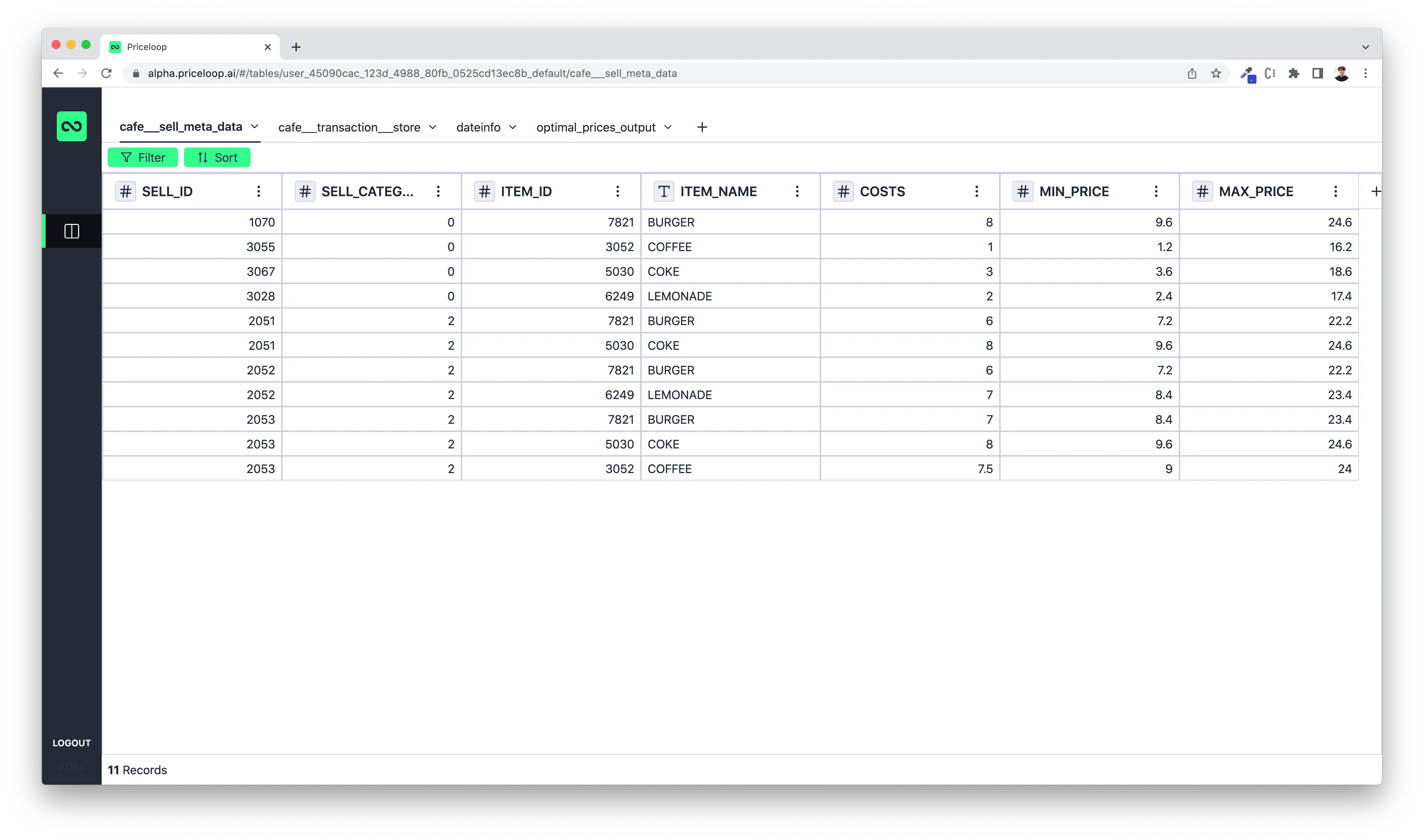
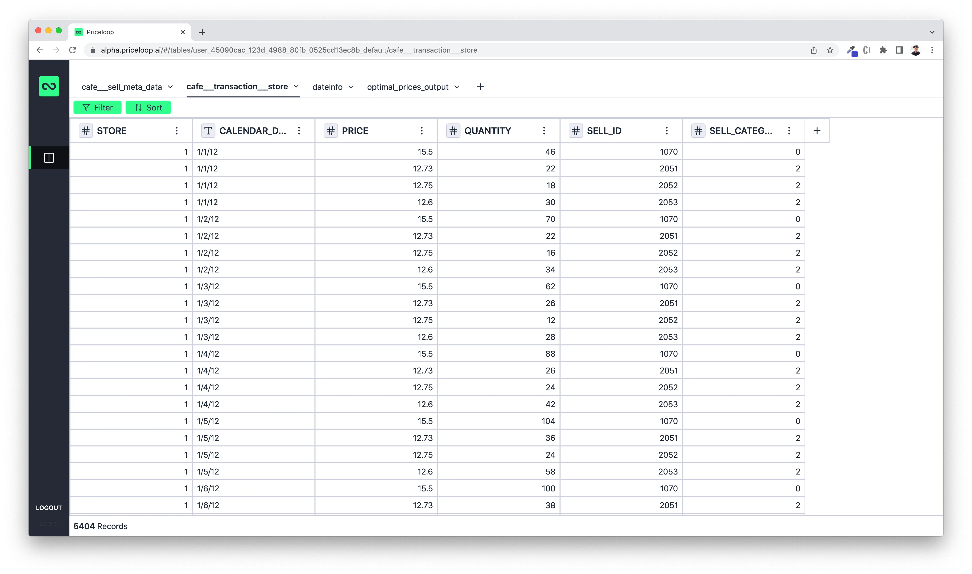
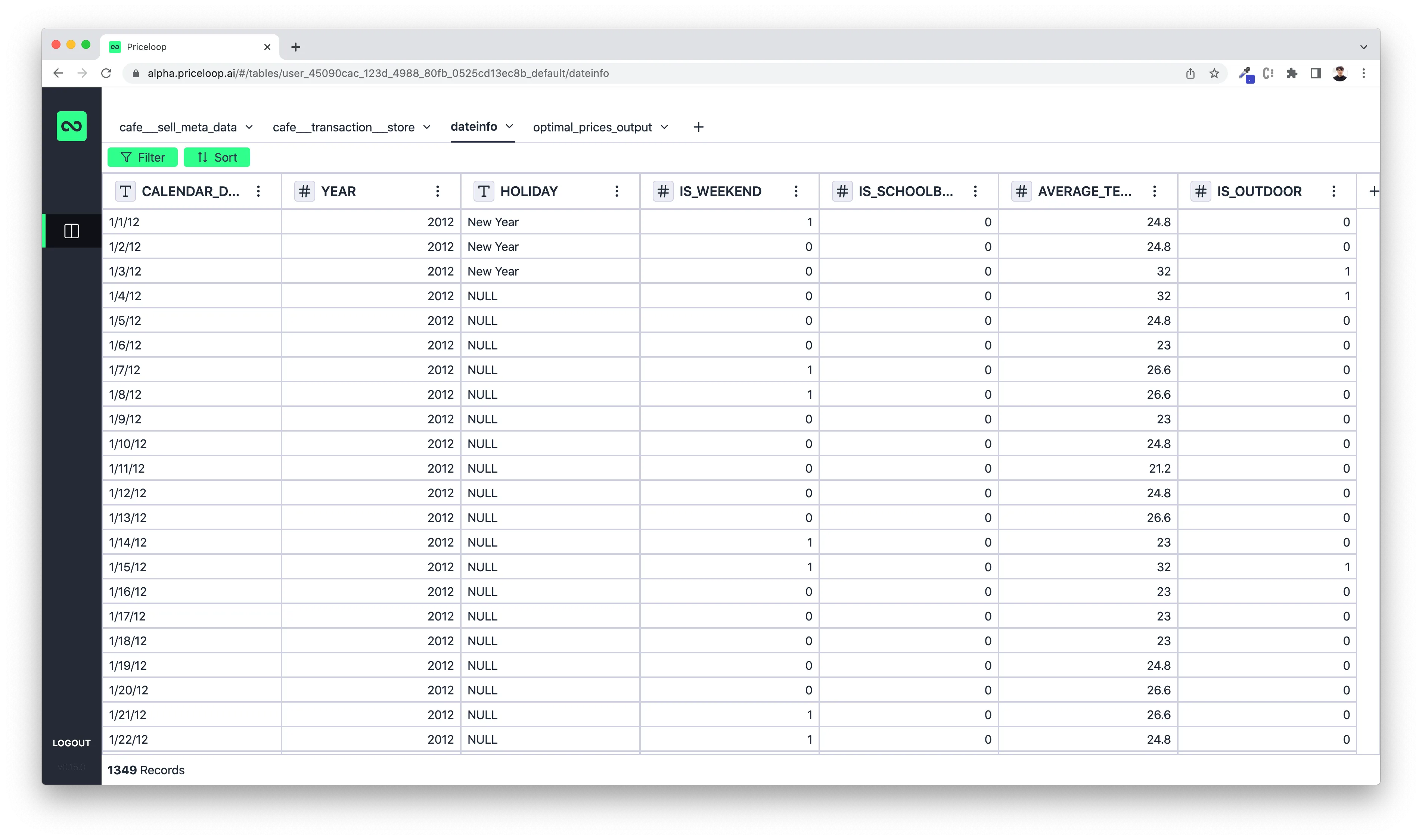
We have already populated the Priceloop NoCode platform with mock data. The data includes categories, sales data, and additional information such as holidays and whether a particular day is a weekend or not.

Here is a preview of the data structure:

‍

Now, your team can seamlessly work with the data by utilizing Priceloop Python API to establish a connection with our platform.

‍

To begin, let's install our library.

pip install priceloop-api

‍

Enter your username and password to establish a connection with the Priceloop platform. While API keys will be employed for authentication in the future, the current authorization method involves using your username and password. Furthermore, we will import all the necessary components for the modeling process.

‍

%matplotlib inline

‍import numpy as np

‍import pandas as pd

‍import matplotlib.pyplot as plt

‍from datetime import datetime

‍from statsmodels.formula.api import ols

‍from statsmodels.graphics.regressionplots import plot_partregress_grid

‍from priceloop_api.utils import DefaultConfiguration, read_nocode, to_nocode

configuration = DefaultConfiguration.with_user_credentials("username", "password")

‍

Now proceed with loading our data:

‍

category_data = read_nocode("cafe___sell_meta_data", configuration, limit=20, offset=0)

transactions_data = read_nocode("cafe___transaction___store", configuration, limit=6000, offset=0)

‍

(Currently, it is necessary to specify a limit and offset when retrieving data. We acknowledge that this process can be more user-friendly, and we have plans to improve it in the near future. The limit parameter determines the maximum of data points to be retrieved, while the offset parameter determines the starting point for data retrieval.)

‍

Creating Machine learning model

After successfully loading the data, the next step involves data cleaning and transformations before proceeding with model building.

‍

# remove duplicates

‍transactions_data = transactions_data.drop_duplicates()

‍# merge category data with sales datadata = pd.merge(category_data, transactions_data.drop(columns=["SELL_CATEGORY"]), on="SELL_ID")

‍# need to group it as we have multiples transactions per day for each SELL_ID

‍cleaned_data = data.groupby(["SELL_ID", "SELL_CATEGORY", "ITEM_NAME", "CALENDAR_DATE", "PRICE", "COSTS"]).QUANTITY.sum()

cleaned_data = cleaned_data.reset_index()

‍

In this straightforward example, we will employ linear regression (OLS) to determine price elasticity.

Let's begin by focusing on a specific product SELL_ID "1070":

‍

burger_1070 = cleaned_data[cleaned_data["SELL_ID"] == 1070]

burger_1070_model = ols("QUANTITY ~ PRICE", data=burger_1070).fit()

print(burger_1070_model.summary())

‍

The regression result is as following:

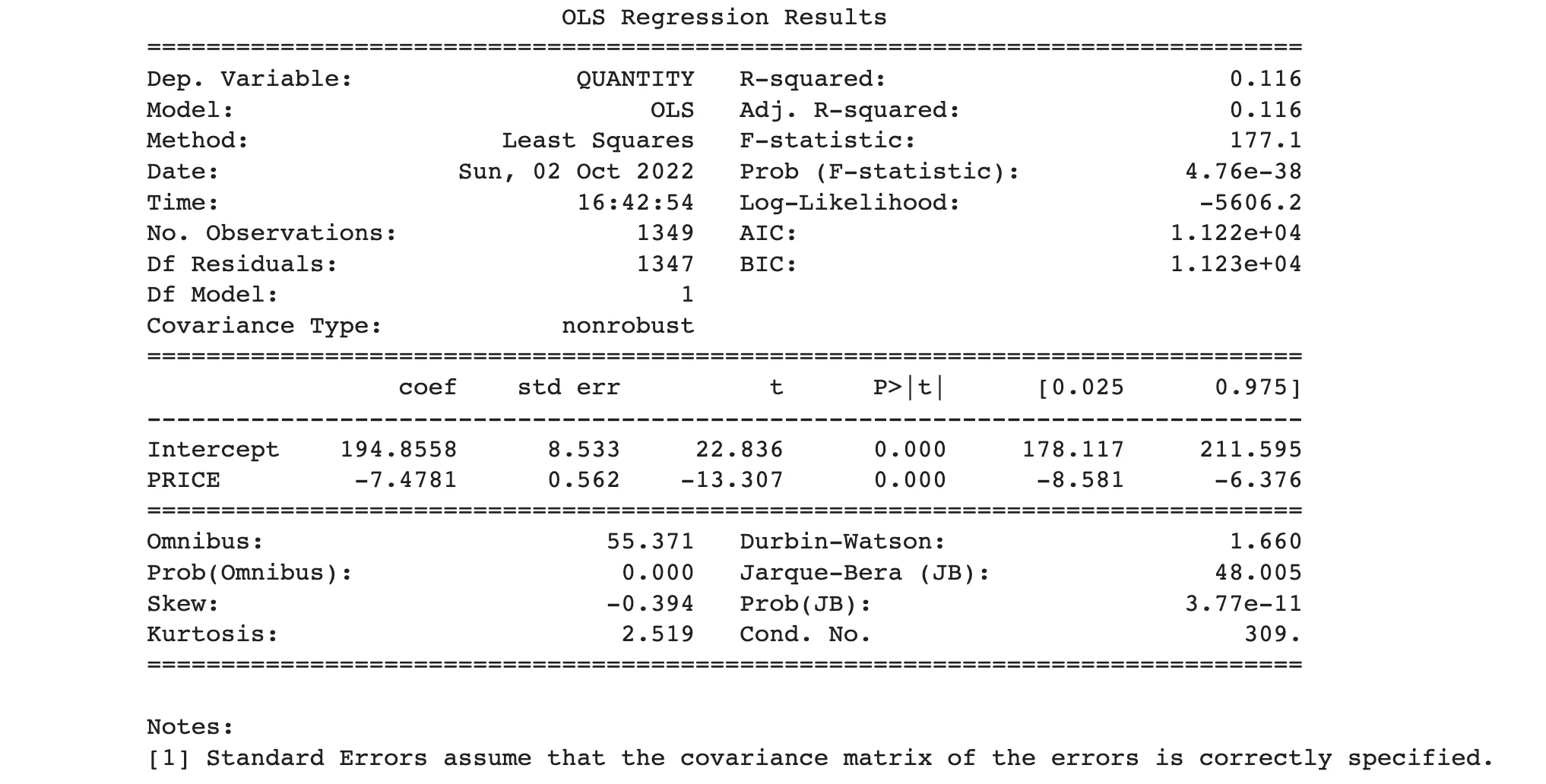
Although the elasticity is approximately -7, the R-squared value is relatively low. In fact, this model does not meet the criteria of a good model, nevertheless, it is essential to understand that the purpose of this article is not to present a high-performing model. Instead, our primary goal is to demonstrate the workflow using our platform.

Now we can apply it to all other products:

model_elasticity = {}

‍def create_model_and_find_elasticity(data):

       model = ols("QUANTITY ~ PRICE", data).fit()

        price_elasticity = model.params[1]

        return price_elasticity, model

‍for i, df in cleaned_data.groupby(["SELL_ID", "ITEM_NAME"]):

       e, model = create_model_and_find_elasticity(df)

       model_elasticity[i] = (e, model)

‍

The output will look like this:

# all elasticities are negative, this is good

‍model_elasticity

{(1070, 'BURGER'): (-7.478107135366496,<statsmodels.regression.linear_model.RegressionResultsWrapper at 0x7fd4fad3af40>),

(2051, 'BURGER'): (-1.9128005756803146,<statsmodels.regression.linear_model.RegressionResultsWrapper at 0x7fd4faa1c8e0>),

(2051, 'COKE'): (-1.9128005756803146,<statsmodels.regression.linear_model.RegressionResultsWrapper at 0x7fd4fae2af40>),

(2052, 'BURGER'): (-2.271811473474679,<statsmodels.regression.linear_model.RegressionResultsWrapper at 0x7fd4fae32be0>),

(2052, 'LEMONADE'): (-2.271811473474679,<statsmodels.regression.linear_model.RegressionResultsWrapper at 0x7fd4fae32490>),

(2053, 'BURGER'): (-5.226102393167906,<statsmodels.regression.linear_model.RegressionResultsWrapper at 0x7fd4fae39490>),

(2053, 'COFFEE'): (-5.226102393167906,<statsmodels.regression.linear_model.RegressionResultsWrapper at 0x7fd4fae40e20>),

(2053, 'COKE'): (-5.226102393167906,<statsmodels.regression.linear_model.RegressionResultsWrapper at 0x7fd4fae47850>)}

‍

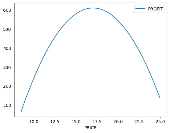
The next step involves identifying the optimal price point that maximizes profit. We will begin this process by focusing on again on product "1070".

‍

burger_1070 = cleaned_data[cleaned_data["SELL_ID"] == 1070]

start_price = 8.5

end_price = 25

opt_price_table = pd.DataFrame(columns = ["PRICE", "QUANTITY"])

opt_price_table["PRICE"] = np.arange(start_price, end_price, 0.01)

opt_price_table["QUANTITY"] = model_elasticity[(1070, "BURGER")][1].predict(opt_price_table["PRICE"])

opt_price_table["PROFIT"] = (opt_price_table["PRICE"] - burger_1070.COSTS.unique()[0]) * opt_price_table["QUANTITY"]ind = np.where(opt_price_table["PROFIT"] == opt_price_table["PROFIT"].max())[0][0]

opt_price_table.loc[[ind]]

‍

In the following graph, it shows that the optimal price is around ~17.

‍

Following shows you how to find the best pricing strategy for all your products.

‍

def find_optimal_price(data, model):

        start_price = data["COSTS"].unique()[0] + 0.5

        end_price = data["COSTS"].unique()[0] + 20

        opt_price_table = pd.DataFrame(columns = ["PRICE", "QUANTITY"])

        opt_price_table["PRICE"] = np.arange(start_price, end_price, 0.01)

        opt_price_table["QUANTITY"] = model.predict(opt_price_table["PRICE"])

        opt_price_table["PROFIT"] = (opt_price_table["PRICE"] - data["COSTS"].unique()[0]) * opt_price_table["QUANTITY"]

        ind = np.where(opt_price_table["PROFIT"] == opt_price_table["PROFIT"].max())[0][0]

        opt_price_table["SELL_ID"] = data["SELL_ID"].unique()[0]

        opt_price_table["ITEM_NAME"] =  data["ITEM_NAME"].unique()[0]

        optimal_price = opt_price_table.loc[[ind]]

         optimal_price = optimal_price[["SELL_ID", "ITEM_NAME", "PRICE"]].rename(columns={"PRICE": "ML_PRICE"})return optimal_price

        optimal_prices = []‍

for i, df in cleaned_data.groupby(["SELL_ID", "ITEM_NAME"]):

        ml_price = find_optimal_price(df, model_elasticity[i][1])

         optimal_prices.append(ml_price)

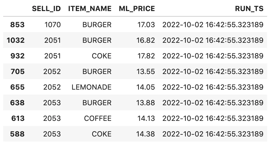
         optimal_prices_output = pd.concat(optimal_prices)

         optimal_prices_output["RUN_TS"] = now = datetime.now()

‍

The output shows as below:

‍

‍

Let's export the result to Priceloop's platform:

to_nocode(optimal_prices_output, "optimal_prices_output", configuration, mode="replace_data")

‍

At present, our API offers four modes: "replace_data", "new", "append", and "recreate_and_delete" (with the latter being the default mode). Considering our specific use case, the best option is "replace_data" because it allows us to incorporate additional logic into Priceloop platform. This ensures that when the data science team retrains the model, all the supplementary logic remains intact within our platform and is not removed.

‍

Implementing additional pricing logic using Priceloop NoCode.

‍

We can now join our data sets and incorporate additional logic in Priceloop NoCode. The exciting aspect is that now, if the pricing manager wishes to modify the minimum/maximum prices or any other pricing/business logic they have implemented, they can do so directly within our platform. Typically, such logics are hardcoded into the code of production systems, requiring IT intervention for modifications.

In the below graph, we add a new formula and join the category table with the table containing the optimal price outputs generated by our data science team. This integration enables us to obtain the minimum prices. Similarly, we follow the same procedure for determining the maximum prices.

‍

Then we check whether our machine learning-generated prices fall within the minimum and maximum price ranges. If the ML price is lower than the minimum price, we would set the minimum price as the final price. Conversely, if the ML price exceeds the maximum price, we would consider the maximum price as the final price.

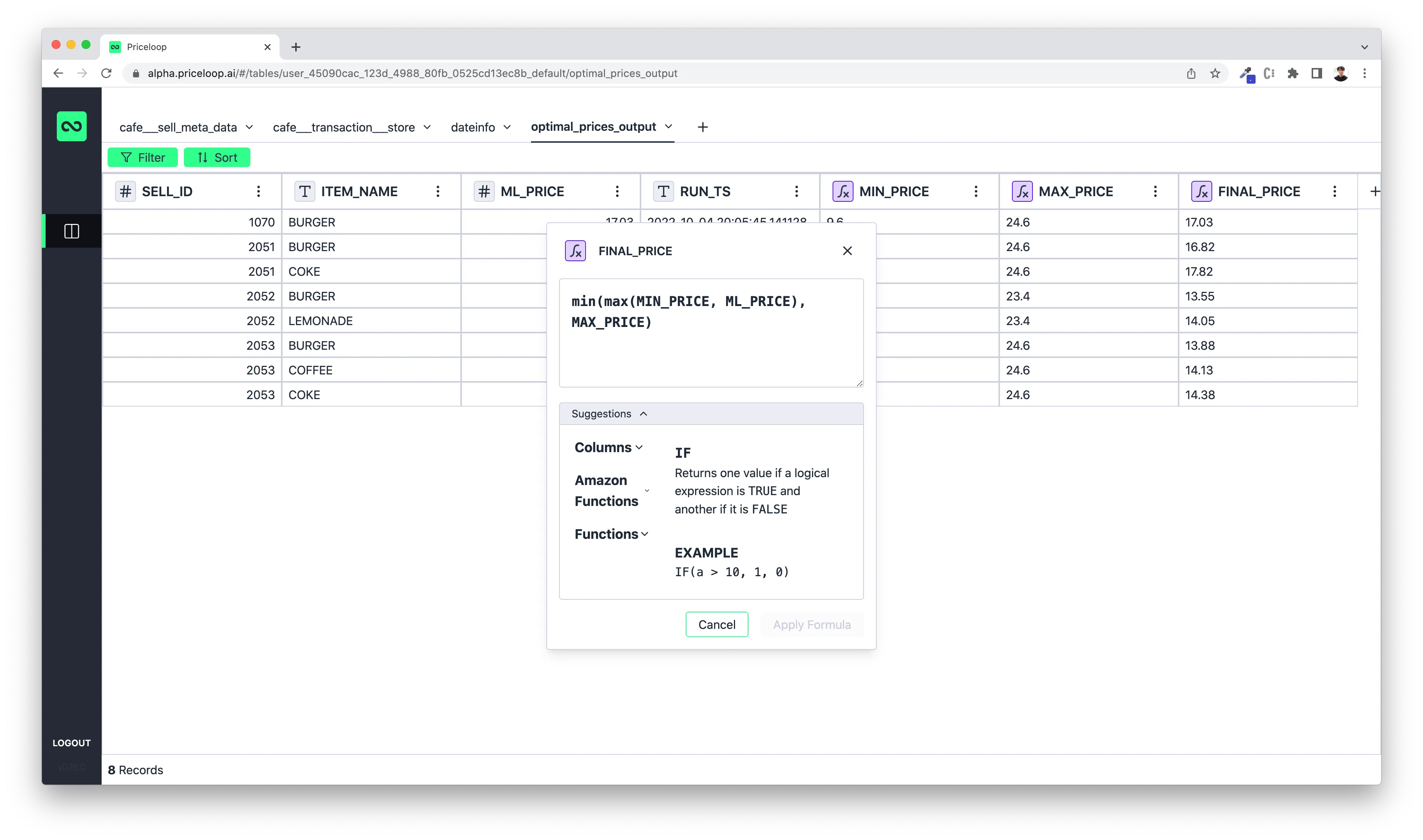
This example is quite straightforward. However, when collaborating with our clients, these types of logic can become considerably intricate, involving numerous functions and intricate chains of operations.

‍

Taking your logic into production

‍

After achieving consensus among all stakeholders, the IT department can apply our API again to import the final output into their production system. Currently, this is the most effective method available. We are actively working on expanding the range of exportable sources to provide additional options in the near future.

‍

from priceloop_api import ApiClient

from priceloop_api.api.default_api import DefaultApi

from priceloop_api.utils import DefaultConfiguration

configuration =

DefaultConfiguration.with_user_credentials("username", "password")

with ApiClient(configuration) as api_client:

         api_instance = DefaultApi(api_client)

          workspaces = api_instance.list_workspaces()

          workspace = api_instance.get_workspace(workspaces[0])

           table = api_instance.get_table(workspace.name, workspace.tables[0].name)

           table_data = api_instance.get_table_data(workspace.name, "optimal_prices_output", limit=100, offset=0)    

           print(table_data)

‍

This article demonstrated the straightforward process of constructing a basic ML pricing optimization model and utilizing our user-friendly Priceloop NoCode platform. We hope you found this article enjoyable and are encouraged to explore our NoCode platform in the near future.